A training set must be selected in the secondary menu in order to activate the classification button.
Button Classify ( Train a Classifier & Classify) trains a new classifier and performs the classification using the algorithm selected in the menu and the specified set of maps.
Once the classification is achieved, a new mask file is generated and stored under Masi files in the secondary menu. The mask file is automatically selected and the mask image displayed in the main figure.
Additional tools: filtering options
The following options apply to a given mask file. Select a mask file in the secondary menu to apply changes.
Select this option to hide pixels having a class probability lower than a given threshold (see below) for the selected mask file.
Set the probability threshold used for hiding pixels (see above). This value should range between 0 and 1.
Button Create new mask file with pixels filtered by probability (all pixels below threshold) generate a new mask file after filtering. This option replaces the BCR correction available in XMapTools 3 and is more adequate as only the miss-classified pixels are excluded.
Additional tools: mask analysis & visualisation
The modes of each class within a given region-of-interest can be exported using the tools provided in this section. Modes are given as surface percentage calculated using the number of pixels of each class. For minerals, it can be eventually extrapolated to volume fraction as discussed in Lanari & Engi (2017).
Menu to select the ROI shape to be used to extract the local modes.
Button Add ROI allows a new region-of-interest (ROI) to be drawn on the figure. Note that a mask file must be selected before activating this mode. Results are displayed in the right window as a table containing the modes and number of pixel for each class and as a pie diagram. Note that the diagram can be saved using the plot options located at the top-right while the mouse pointer is over the plot.
The following ROI shapes are available:
- Rectangle: click to select the first corner and drag the mouse to the opposite corner defining a rectangle
- Polygon: click successively on the image to draw a polygon; right-clicking validates and closes automatically the shape
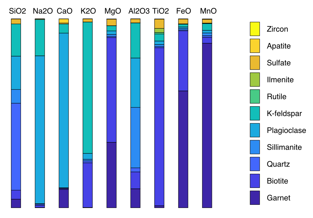
Button Plot Compositions generates a plot using the data selected in the primary menu (either intensity, or a merged map) and the mask file selected in the secondary menu. An example is given in Figure 2.
Was this helpful?
1 / 0