The new approach implemented in XMapTools 4 provides a module for auto multi-phase calibration. Note that this is a preliminary version of the calibration assistant. We are expecting significant progress in the coming years once the algorithm is trained to face the most challenging situations. In the same time, please contact Pierre Lanari (pierre.lanari@geo.unibe.ch) if your case is not handled well by the algorithm.
Table of Contents
Strategy advantages and pitfalls
An auto calibration was performed considering all spot analyses and all masks when you pressed the button Calibrate. The new algorithm performs first a general fit including all standards and then adjust the calibration for each mineral. All calibration curves, including those for the general fit are accessible via the tree menu.
If you press the button Apply Standardization, all calibrated maps, for each mineral as well as a merged map are created and sent back to XMapTools. It seems magic, but it is not so first make sure that you check the quality of the calibration curves determined by the auto function.
The auto function works if all minerals have been measured with at least a few spot analyses and if there is at least one mineral with a composition above 1 wt% for each element. If a mineral or other feature (e.g. fracture) have no spot analyses, the program extrapolates a calibration from the general fit, therefore “predicting” a composition. At this stage, this composition is likely to be wrong because of matrix effects are ignored!
If you close the Calibration Assistant window neither calibrated data or calibration settings are saved.
If you press Apply Standardisation all maps are sent to XMapTools.
Procedure description
The Calibration Assitant For EPMA Data opens after the button Calibrate in XMapTools was pressed.

Displaying calibration curves
Use the tree menu located on the left side to navigate through the list of minerals and elements and to display calibration curves.
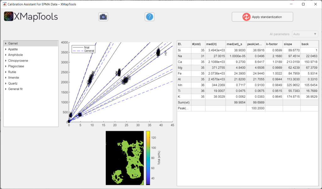
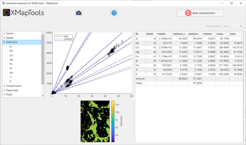
if you select a mineral in the tree menu (Figure 1). A single map showing the sum of elements/oxides (total wt%) is displayed. The plot in the central part shows all calibration curves, for all the elements of the selected mineral. Some data are showed in a table.
- El. shows the element name (of the map), the total of the median mineral composition considering all pixels (sum(wt%)) and the total of the peak position (Peak(SumOx))
- #(std) shows the number of internal standards used for calibrating this phase (e.g. 42 spot analyses for amphibole in Figure 2). Some elements may have smaller number of internal standards because of outlier rejection
- med(it) shows the median intensity value of the selected mineral for each element
- med(wt)_s shows the median standard composition (spot analyses)
- peak(wt)_m shows the median composition of the calibrated map. Note that the values of Peak(SumOx) and Sum(Wt) can be different, in this case the median value is probably affected by non-gaussian signals and may not compare with the median of the spot analyses. Yet comparing both columns can be used to detect potential calibration problems to be fixed using the manual adjust (see below).
- k-factorquantifies the difference between the calibration obtained during the general fit and the final calibration of the selected mineral. A value of 1 means that both are identical
- Slope of the calibration curve of each element.
- Background value for each element.

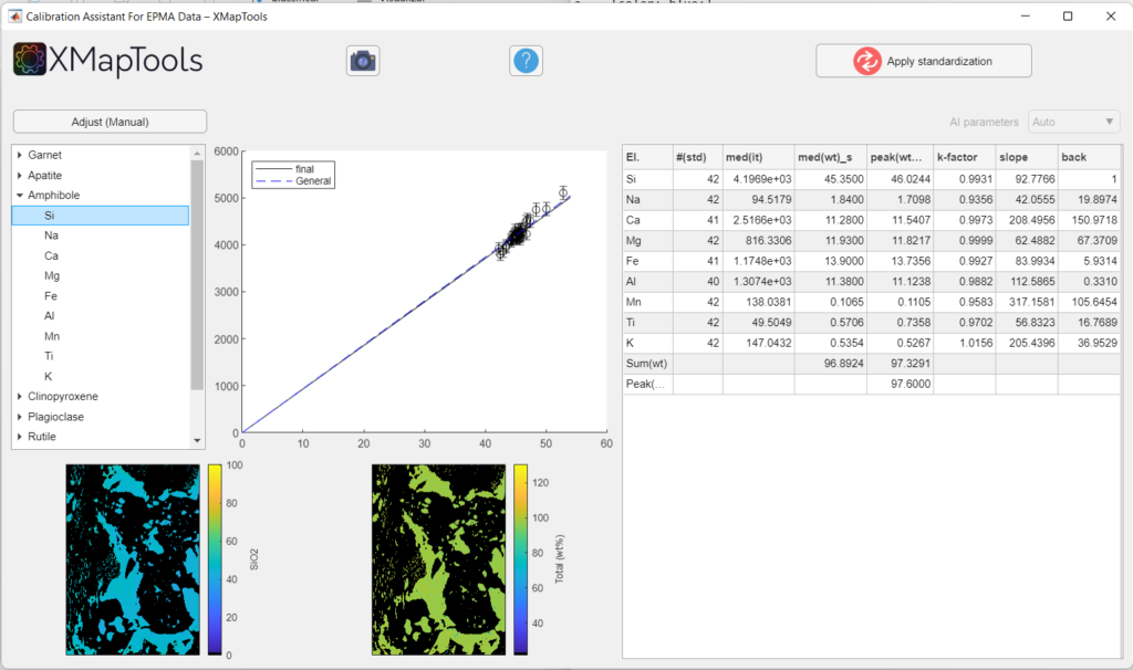
To display a specific calibration curve (for a given element), unfold the menu by clicking on the small arrow on the left side of the mineral name and select an element. The corresponding calibration curve is displayed as well as the correspondent quantitative map (oxide wt-%) (Figure 3).

Adjusting a calibration curve
When an element is selected the button Adjust ![]() appears above the tree menu.
appears above the tree menu.
Clicking on this button display two fields containing the values the values for background and slope:

Values can be changed manually by tapping new values in the corresponding field.
Press enter to calculate and display the new calibration curve on the plot (this operation can take a few seconds).
Displaying results of the general fit
By selecting the General fit (last option in the tree menu, Figure 3), a plot with the calibration curves for all the elements are displayed.
No adjustment on the calibration curves in the general fit is possible. This fit is automatically performed first by the program and no longer used once the calibration of each mineral is achieved.
Apply calibration

After checking each calibration curves and adjusting, if necessary, use the button Apply standardization to generate the calibrated maps.
By applying the standardization, the option Quanti in the Primary Menu becomes available. There, the quantitative maps in element/oxide wt-% of each phase can be displayed.
The option Merged in the Primary Menu also becomes available after the standardization. A set of merged maps (i.e., quantitative maps in oxide wt-% for all the phases considered together) is automatically generated.
Notes
Red spots show outliers that are not considered in the calculation of the calibration curves.
By hoving the cursor on the images an image menu will appear on the upper right. This menu includes options to zoom, save and copy the images.
References
- De Andrade, V., Vidal, O., Lewin, E., O’Brien, P., Agard, P., (2006). Quantification of electron microprobe compositional maps of rock thin sections: an optimized method and examples. Journal of Metamorphic Geology, 24, 655–668.
- Lanari, P., Vho, A., Bovay, T., Airaghi, L., Centrella, S., (2019). Quantitative compositional mapping of mineral phases by electron probe micro-analyser. Geological Society of London, Special Publications, 478, 39-63.
- Tedeschi, M., Lanari, P., Rubatto, D., Pedrosa-Soares, A., Hermann, J., Dussin, I., Pinheiro, M.A., Bouvier, A.S., Baumgartner, L. (2017). Reconstruction of multiple P-T-t stages from retrogressed mafic rocks: subduction versus collision in the Southern Brasília Orogen (SE Brazil). Lithos, 294–295, 283–303.
Was this helpful?
1 / 0